Background

We will start by introducing the necessary background ideas to understand what is happening. First we will introduce the notion of a map, by giving an analogy to differential equations (DE). A system of DE's is a set of equations which tells how some things change with respect to some other variable. For example, the equation:

tells us how the variable x, which represents the position of a particle, changes with respect to time. This is a continuous relationship, so for any time t, there is a value for . The idea of maps is very similar, but now the relationship is discrete. Things no longer change continuously, but in steps. A differential equation can be regarded as a difference equation in a limit as the space in between the steps goes to zero. A map is like this, but there the space in between the steps is fixed and finite. Let's look at a simple example.

So now is not a function of a continuous variable, but we get the value for x at different steps n. Just like a differential equation, we start off with an initial condition, say =1 in our example. Now plug this in and we get =2. Now plug this back in again and we get =3 and so on. This process is called iterating the map. This is the basic idea of a map and while it might seem redundant now, keeping this idea in mind will help make things clearer later.

Now we introduce some other notions which will also be necessary. One key idea is the notion of a fixed point. A fixed point is a point which does not change under iteration of the map; specifically, . This is what is called a period one fixed point. Fixed points of higher period occur as the map is iterated. For example, suppose , but . In this case, we say is a point of period k. It is easy to see from this that a set of period n points will contain all the points of period k, when k|n. Again for example, the set of all period six points for some map will contain all the period one, two and three points, plus some extra points which are specific to the period six.

We ask, what good is a fixed point? Linearization about a fixed point tells us the behavior in the neighborhood of the point. Points near the fixed point act in one of four ways, depending on the nature of the fixed point. If you start at a point in the neighborhood of the fixed point and iterate the map at that initial point, the behavior of the solution will either fall into the fixed point (in which case it is called a sink), move away from it (a source), experience a combination of those two (a saddle) or revolve around it in an orbit (a center). This is illustrated in Fig.1, where the lines represent the behavior of a solution as time goes on.

 
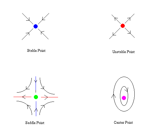
Figure 1:   Behavior in the Neighborhood of Fixed Points

A useful technique to determine the behavior near a fixed point is to linearize the equations of the map about that fixed point. We can then write these equations in matrix form, which we call the Jacobian (we will call it the matrix A later). You can then find values called the eigenvalues of this matrix. We do this by finding the determinant of the difference between the Jacobian and a matrix which is all zero except for 's along the diagonal. Specifically, we have an equation which looks like where I is the identity matrix. It is these values which are our eigenvalues. Depending on how many dimensions your system is, you might get a complicated expression for . For example, if you have a three dimensional system, will be the root of a cubic equation, which might be easily solvable or it might not.

These eigenvalues tell you the stability of the fixed point as prescribed above. If the absolute value of the eigenvalues is less than 1, then the fixed point is a sink. If they are greater than 1, the fixed point is a source. If they are a combination of these, the fixed point is a saddle. If they are exactly equal to 1, then the fixed point of the linearized system is a center, and the quadratic terms control the behavior. The behavior of the map in neighborhoods of periodic points can be characterized in the same way as fixed points

This might be confusing so let's look at an example and see how we can use the machinery defined above. Let's look at the system . This is a two dimensional map and can be thought of as the system:

Now as specified above, we will have a period one fixed point when and . Using a substitution and a little help from the quadratic formula, we see that this occurs when (x,y) = (0,0) or (3,9). So we have two period one fixed points for our system. As noted above, these will always be fixed points, so we are interested in their stability. Let's look at the point (x,y)=(3,9). If we can find the eigenvalues for this point, then we will have a sense for the behavior of points nearby (3,9). So let's look at an arbitrary point close to the fixed point. Let and where and are numbers very close to zero. We want to plug these into the equations and eliminate x and y. So for example, we would write . Working out the algebra, we get a system which looks like:

Now we have a nice system which tells us the behavior close to the fixed point. Since we are close by, we can neglect all higher order terms and only look at the linear terms. So we write out this system in matrix form:

This is our linearized system in matrix form, where the matrix A is the Jacobian for that point. So now we want to solve the equation to get the eigenvalues. So we have:

This gives values for of 3 and -2. The absolute value of these numbers is greater than one, so our fixed point is unstable. This tells us that points near (3,9) will diverge away from that point as we iterate the map. This example may seem a bit long winded, but it serves to show how the basic machinery works. The same technique can be used to find the stability for any fixed point of any period.

Another useful technique to look at is the idea of a bifurcation. When we have a system, there are certain parameters which can be varied. For example, let's take a look at the quadratic map, which will one of the main focuses later on. The map is given by the equation:

Where a is a constant. Since a can be any constant number, changing its value will have the effect of changing the fixed points and their associated eigenvalues. So the inherent behavior of the system depends on the value for this parameter. We call this a bifurcation parameter. We can write a program which iterates the map for a certain value of a, assuming we give an acceptable initial condition for . If we start off at too large a value, the iterates will diverge off to infinity and we get nothing interesting. But if we stay in an acceptable range where is small enough and make a plot of the iterates as a function of our bifurcation parameter a, we get an interesting pattern. This is called the period doubling cascade, as shown in Figure 1. This shows us that the number of fixed points in the system grows faster and the complexity of the system increases.

 
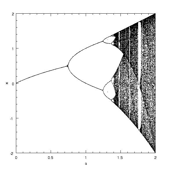
Figure 2:   Period Doubling Cascade For the Quadratic Map

We see that solutions tend towards the stable fixed point for small values of a. But as a increases, we get more and more periodic fixed points. stops moving towards a single stable orbit, and starts being pushed about by various unstable high-period fixed points. This is a signature of chaos.

What does it mean to have chaos? Well the simplest way to define a system as chaotic is if we see a sensitive dependence on initial conditions. This means that if we start at some initial point and iterate a bunch of times, then take a point arbitrarily close but not the same point and iterate the same number of times, the two can be very different. A good example of a chaotic system is the weather. A small change somewhere can cause a big change somewhere else. For example a butterfly flapping it's wings on a Pacific island causes a thunderstorm in Toronto five years later.