The basic one dimensional quadratic map is given by:
![]()
Where a is a constant and also acts as the only bifurcation
parameter for the system. The period one fixed points are found
setting ![]() :
:
![]()
We can see that for fixed points to exist, ![]() because x is a real map and thus a fixed point cannot be
complex. Now we can go a couple steps further and find the higher
period points. The period two points are given by:
because x is a real map and thus a fixed point cannot be
complex. Now we can go a couple steps further and find the higher
period points. The period two points are given by:
![]()
We see once again that there is a constraint on a for the existence
of period two points, namely ![]() . This observation
leads one to wonder, what values of a lead to higher period orbits?
The plot above shows stable orbits of higher period developing for
increasing a. At high enough a, we see the situation which is
referred to as chaos: any two initial points, no matter how
close, will eventually diverge.
. This observation
leads one to wonder, what values of a lead to higher period orbits?
The plot above shows stable orbits of higher period developing for
increasing a. At high enough a, we see the situation which is
referred to as chaos: any two initial points, no matter how
close, will eventually diverge.
This brings us to the main focus of this paper: given two independent systems which vary slightly in initial conditions, we seek a way to modify the systems so that they do not diverge under iteration. One proposed solution is as follows, namely the coupled system:
![]()
We have effectively changed the pair of one dimensional maps into a two
dimensional map. The system is uncoupled when the parameter ![]() , that is to say that the two systems act independently. The goal
is to keep these two systems as loosely coupled as possible, but
still have them synchronize. By this we mean that
, that is to say that the two systems act independently. The goal
is to keep these two systems as loosely coupled as possible, but
still have them synchronize. By this we mean that ![]() . We call this
synchronizing the two chaotic systems. The first method of attack on this
problem is analytical. For a given a, we want to find values of
. We call this
synchronizing the two chaotic systems. The first method of attack on this
problem is analytical. For a given a, we want to find values of
![]() so that for close initial values of x,y, synchronization
must occur. To simplify this task, we introduce the new variable
so that for close initial values of x,y, synchronization
must occur. To simplify this task, we introduce the new variable
![]() , and we are interested in when
, and we are interested in when ![]() . Through a little algebra, the map becomes:
. Through a little algebra, the map becomes:
![]()
Since ![]() depends on x, we want to get some idea of when x
itself remains bounded. In other words, we want to solve for b
such that
depends on x, we want to get some idea of when x
itself remains bounded. In other words, we want to solve for b
such that ![]() (that is,
(that is, ![]() ). When x is at the maximum value of b, we get
). When x is at the maximum value of b, we get ![]() , and the
solution
, and the
solution ![]() . On the other hand,
|a| must not exceed b or else when
. On the other hand,
|a| must not exceed b or else when ![]() , then
, then
![]() . This leads us to the requirement
. This leads us to the requirement ![]() .
Unless this is satisfied, all solutions which do not start out at a
fixed point eventually diverge. The information just obtained is
useful in understanding the 1D quadratic map, but now we wish to
apply it to the coupled system. We ideally would like
.
Unless this is satisfied, all solutions which do not start out at a
fixed point eventually diverge. The information just obtained is
useful in understanding the 1D quadratic map, but now we wish to
apply it to the coupled system. We ideally would like ![]() . Thus we impose the condition
. Thus we impose the condition ![]() , which can be satisfied using the triangle inequality and
our bound on
, which can be satisfied using the triangle inequality and
our bound on ![]() as follows:
as follows:
![]()
By assuming that our initial ![]() is arbitrarily small (remember
we only need to show synchronization for small initial differences),
we can neglect
is arbitrarily small (remember
we only need to show synchronization for small initial differences),
we can neglect ![]() and proceed:
and proceed:
![]()
Substituting an ![]() in this range into the above, we find the range of
in this range into the above, we find the range of
![]() for which synchronization is guaranteed:
for which synchronization is guaranteed:
![]()
It is reassuring to know that given a quadratically coupled map,
there is a coupling parameter which will force synchronization for
small enough initial variations. However, plugging in various a
in the range [1.5,2.0], where interesting behavior occurs, we find
that the analytically obtained values of ![]() are between roughly
0.28 and 0.25. Remembering that lower
are between roughly
0.28 and 0.25. Remembering that lower ![]() means stronger
coupling, we see that these are very strongly coupled systems. The
question arises, can we improve on this result? After all, two very
restrictive relations were used, namely the maximum value of
means stronger
coupling, we see that these are very strongly coupled systems. The
question arises, can we improve on this result? After all, two very
restrictive relations were used, namely the maximum value of ![]() and the triangle inequality.
and the triangle inequality.
The answer to this question may be sought through numerical methods. One such method is DSTOOL, a software package which allows us to see fixed points, periodic orbits, and stable and unstable manifolds, which are the points that fall into and ``originate from'' (in the sense that they fall in under the inverse map) the fixed point. DSTOOL was used mostly for these tasks, as well as to look at the iterations of specific initial points.
The second technique was a bit more involved. The most direct test
for synchronization is to iterate the map several times, and see if
for a given point ![]() approaches 0. By breaking the plane
into a fine grid, and iterating at each point in the grid, we can
obtain a fairly good picture of the synchronization of the system.
This was done using a FORTRAN program, and the results were fairly
interesting. As the diagrams below show, there is good
synchronization for coupling much weaker than the analytic work
would indicate. Further, there is a distinct critical threshold of
approaches 0. By breaking the plane
into a fine grid, and iterating at each point in the grid, we can
obtain a fairly good picture of the synchronization of the system.
This was done using a FORTRAN program, and the results were fairly
interesting. As the diagrams below show, there is good
synchronization for coupling much weaker than the analytic work
would indicate. Further, there is a distinct critical threshold of
![]() at which the basin of attraction loses its connectivity.
The synchronization near this value of
at which the basin of attraction loses its connectivity.
The synchronization near this value of ![]() appears to be highly
sensitive, as the following diagrams show for the value a = 1.5,
which is in the chaotic regime.
appears to be highly
sensitive, as the following diagrams show for the value a = 1.5,
which is in the chaotic regime.
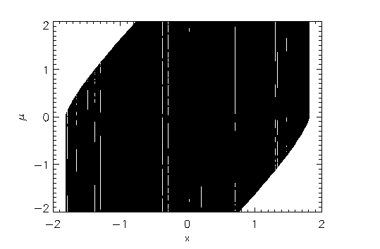
Figure 3: Basin of Attraction; a = 1.5, ![]() ,
, ![]()
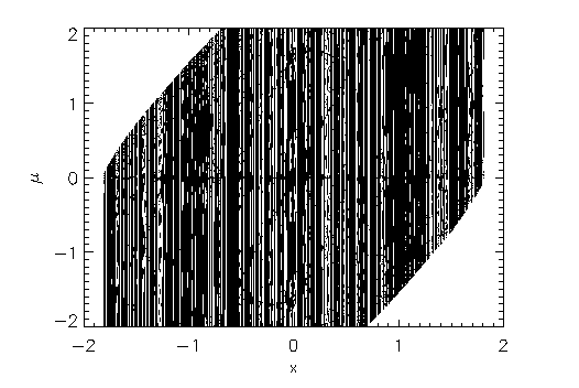
Figure 4: Basin of Attraction; a = 1.5, ![]()
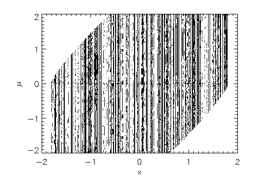
Figure 5: Basin of Attraction; a = 1.5, ![]()