We will begin our analysis by examining how the trajectories of the system
change over time. That is, we
will start with a given point in the system (that is, with certain
e and n values) and see how that point moves over time.
Figures [1(a)-(b)] show the orbits when begun from a non-zero e
value ( ![]() ), and n = 0. (Other orbits are similar).
), and n = 0. (Other orbits are similar).
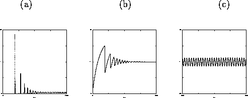
Figure 1: (a) Changes in the amplitude |e| vs. time. (b): Changes in the number of the carriers n vs. time. (c) ![]() vs. time.
vs. time.
These graphs were obtained using DSTool, a computational analysis tool,
using the ![]() and
and ![]() equations described earlier ((7) and (8)).
The following parameter values were used:
equations described earlier ((7) and (8)).
The following parameter values were used:
![]()
![]()
![]()
J = 0.0859794
![]()
c = 1
These values represent realistic parameter values for the laser.
Looking at Figures [1(a)-(b)], we see that at first, n climbs steadily, while |e| drops immediately towards (but does not actually reach) zero. At a critical value, n takes a sharp drop, corresponding to a jump in |e|. The lasing has begun. This initial burst of energy in the field is shown in Figure [1(a)]. Notice that this burst of energy (that is, increase in the amplitude), corresponds exactly with the sharp drop in n shown in Figure [1(b)].
The carrier density, n, begins to build up again (and |e| drops
again),
but this time, the critical value of n is not as high, and |e| does
not
drop as low. A series of drops occurs until n and |e| reach a balance.
Then, n appears to stop moving (in actuality, the rate of gain and loss
in the ![]() equation have balanced out), while e spins
clockwise on the complex plane (
equation have balanced out), while e spins
clockwise on the complex plane ( ![]() vs.
vs. ![]() ) at a constant
radius. (That is, |e| is a constant.) This periodic behavior is shown in
Figure [1(c)]. This is typical behavior for a laser, a sign that
our model is a good one.
) at a constant
radius. (That is, |e| is a constant.) This periodic behavior is shown in
Figure [1(c)]. This is typical behavior for a laser, a sign that
our model is a good one.
Let us now change the parameter values and observe how the change affects
the system. We will lower the "pump" term, J to 0.03, and recalculate
the trajectories of the system, using the same starting point
( ![]() , n = 0).
, n = 0).
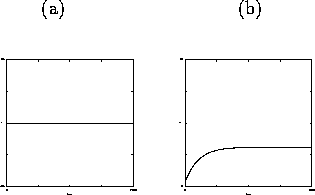
Figure 2: Changes in the (a) amplitude |e| and (b) number of carriers vs. time, J = 0.03
With the low "pump" term, n never becomes large enough to reach a critical value, as we saw before. Thus, there is never a corresponding increase in |e|. Therefore, instead of approaching a periodic solution, e approaches 0. This, too, is typical behavior for a laser: if the "pumping" energy level is too low, the laser cannot operate, as the carrier density never becomes high enough for lasing to begin. This will become clear in the bifurcation diagrams of the system, presented later on in this paper.